Data-based Equation for the Directional Quanta at the 1st Moment
In the prior article we derived the values of the Living Average's quanta of info energy. It turned out that one equation determines the value of every Living Average quanta. The Living Average is the Living Algorithm's 1st derivative. Every Living Algorithm derivative has info quanta associated with it, not just the 1st. However, only the Living Average Grid has quanta of info energy. The rest of the info quanta are in relationship to the Living Average's info energy. For instance, the info quanta of the Living Algorithm's 2nd derivative (the Directional) represent the acceleration of the quanta of info energy from the 1st derivative (the Decay Average). With these distinctions in mind, let us proceed forth.
The Info Quanta of the Directional
At right is a visualization of the info quanta of the Living Algorithm's 2nd derivative, the Directional. While the Living Average is the data stream's velocity, the Directional represents the data stream's acceleration. The Directional is of particular importance due to its intimate relationship with the Active Pulse, a.k.a. the Pulse of Attention. The Active Pulse is a visualization of the Directional of a data stream consisting solely of ones. Accordingly, the Active Pulse is a picture of the data stream's acceleration, the Directional. As mentioned in prior articles, data stream acceleration is at the foundation of force, work and power. At right are the info quanta associated with the first 20 data points of the Active Pulse. Let's deconstruct the Living Algorithm's Directional to see what we can uncover about these info quanta.
The Data-based Equation for the 1st Directional
2.1. Below is the general equation for the Basic Directional - the one that is at the heart of the Pulse of Attention. (The Liminals are higher level Directionals.)
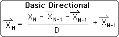
This is a context-based equation, as it contains composite measures, such as the prior Living Average and prior Directional. This form is perfect for living systems, as they must constantly adjust to the context of their situation. However, we aren't adjusting to context, but are instead interested in the content of the equation - the actual data. We are hoping that the content of the equation will reveal something about the info quanta. Hence we are looking for content-based equations to describe the Directional. Our quest is to eliminate all composite measures from our equation. We want to take off all the hats.
2.2 Here is another version of the Directional Equation. For clarity we combine the past Directional into one term and employ K the scaling factor, instead of the clumsy (D-1)/D.
![]()
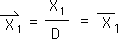
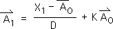
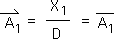
2.3 Let's start with Directional for the first data point, X1, in the stream. Applying the above general equation to the specific yields this result.
![]()
2.4 The Living Algorithm digests the 1st data point to create a Directional, X1 with the arrow on top. Because this is the first data point there are no prior measures. In other words, all prior measures equal zero. This is a given.
![]()
2.5 All the prior measures, the terms with a subscript of 0, drop out of the equation. This is resulting simplification. The Directional at the 1st moment (N = 1) equals the Raw Data, X1, divided by D, the Decay Factor. This is the same value as the Living Average of the 1st moment (Equation 6).
General Derivation: Data-based Equation of the Directional at the 2nd Moment
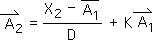
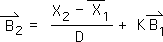
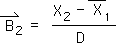
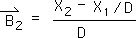
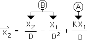
2.6 Now let us derive the data-based equation for the Directional at the 2nd moment in time. Employing general Directional Equation 2:2 we obtain the context-based equation for the Directional at the 2nd moment (N = 2) after the 2nd data byte, X2, enters the System.
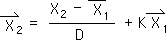
2.7 Substituting the data-based values (Equation 2:3) for our X1s with hats (a bar and an arrow) into the above equation yields this expression.
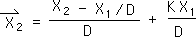
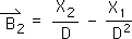
2.8 Performing some standard algebraic manipulations yields the following equation. This is the content-based (data-based) equation for the Directional at the 2nd moment (N=2) that we are looking for.
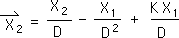
2.9 Look us compare it with its counterpart, the Living Average of the 2nd moment.
![]()
2.10 It is evident that the Living Average and Directional for the 2nd moment are identical except for one term. Subtracting the two yields the term that is the difference.
![]()
Remember that the Living Average and the Directional for the 1st moment are identical (Equation 2.5). Accordingly this intriguing term represents our first point of departure between the two Living Algorithm measures. It won't be the last.
Points of Note
There are a few points of note.
1) This is the first time we've seen a negative sign ('–') in our derivations. The Living Average Grid is completely additive. The info energy quanta combine to produce the Living Average at any moment in the data stream. In other words, there is no such thing as negative energy in the Living Algorithm System. Accordingly, all the info quanta in the Living Average Grid are positive.
2) An inspection of Equation 2.10 reveals that a positive number must be subtracted from the Living Average to yield the Directional. Hence, the Living Average will always be greater than the Directional at the 2nd moment.
3) We still don't know the values of the acceleration quanta.
Event-based Derivation: Data-based Equation for the Directional at the 1st Moment
2.11 To calculate the values of the individual acceleration quantum, we must break the Directional into Events. We begin by applying the general Directional (Equation 2:1) to the 1st Event (A).
2.12 Because this is the 1st moment in the 1st event, there are no prior moments. In other words, the prior Living Average and prior Directional (the X's with hats and a subscript of 0) equal 0. This is a given.
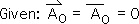
2.13 The terms that equal 0 drop out of the equation, leaving us with this simplicity.
It seems that the 1st term in the 1st event, whether Living Average or Directional, equals the same algebraic expression – the initial byte of raw data, X1, divided by D, the Decay Factor.
2.14 This is also the value of the Living Average (bar) and Directional (arrow) of the 1st moment (Equation 6). Remember we defined the initial moment in any Event as an Impact.
This congruence is not so mysterious. Remember the sum of the Events at a particular moment, N, equals the value of the data stream derivative at that same moment. The data stream's 1st moment (N = 1) is only comprised of Event A. Accordingly, the derivatives of the 1st moment equals the value of Event A at this moment. The info quanta of the 1st moment are Impacts, by definition.
Event-based Derivation: Data-based Equation for the Directional at the 2nd Moment
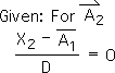
2.15 Now let us look at what happens to the 1st Event on the 2nd Moment, A2 arrow. Note: as the Event's second moment, this info quantum is an Influence. We first apply the context-based Living Algorithm (Eq. 2.2).
Recall from an earlier discussion that the Impacts and Influences of Events are associated with different parts of the Living Algorithm (Equation 34 shown below).
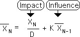
The 1st term determines the value of Impacts, the 1st moment in any Event. The Impact of the Present Instant is the name of the 1st term in the Living Algorithm. The 2nd term determines the value of Influences, the subsequent moments in any Event. The Influence of Past Moments is the name of the Living Algorithm's 2nd term. When we add the 2 terms (the Impact of the Present Instant to the Influence of Past Moments) we get the Present Moment.
Our argument went as follows. An Event's initial Impact has no Past. Therefore, the Present Instant (the 1st term) is the sole determiner of its value. An Event's subsequent Influences have no Present (no more changes). Hence, Past Moments are the sole determiner of their value.
Remember the Present Moment has a host of derivatives associated with it, including the Living Average (the data stream's 1st derivative) and the Directional (the 2nd derivative). This analysis applies to all the data stream's derivatives.
2.16 In the current case, we are dealing with the 2nd moment in Event A, which by definition is an Influence. Accordingly, the Living Algorithm's 1st term (the Present Impact) has no part in determining its value. In other words, it is a given that this Living Algorithm's 1st term always equals zero when speaking of Influences.
2.17 This leads to the expected result – the value of the initial Event scaled by K. No surprises here. In fact, both the Living Average and the Directional for Event 2A have identical values.

2.18 How about the 2nd Event (Event B). Here is where it gets tricky. Applying the Living Algorithm yields:
2.19 Because this is the 1st moment of Event B (the Impact), there are no prior moments, hence no prior Directionals. Accordingly the final term in the equation equals zero.

2.20 This leaves us with the following expression.
2.21 Substituting the data-based value for the Living Average at the 1st moment (Equation 2.14) yields:
2.22 A simple algebraic manipulation produces the data-based equation for Event B's Directional (the arrow) at the 2nd moment.
2.23 Remembering that the sum of the Events at a particular moment (in this case N=2) equals the value of the total Measure (the Directional – the Xs with arrows).
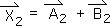
2.24 Substituting the appropriate values from Eq. 2.22 and Eq. 2.17 produces the following equation. As a cross check, this expression is the same as the one we obtained in Eq. 2.8 by a different path (general rather than Event-oriented). We can now determine the individual values of the info quanta (the colored rectangles) at the second moment. The contributions of each Event to the Directional (the acceleration) of the 2nd moment are specified below.
The first time a data byte influences an Event other than its own.
The deceptively simple representation hides a stunning occurrence. For the first time the data from one Event exerts an influence on a subsequent Event. This situation never occurred in the Events associated with the Living Average. This is why we could write one general equation that generated the value for every single quantum of info energy in the Living Average Grid. In contrast, the Events in the Directional Grid are beginning to cross-pollinate. In other words, Event A's data byte, X1, exerts an influence upon Event B's Directional, but not on Event B's Living Average. This is just the beginning of complexity in the midst of the simplicity of the Living Algorithm's digestion process.
Link
We’re not sure whether the Directional’s 3rd moment will result in more complexity or a simplification. For the algebraic results, check out the next article in the series: Directional Quanta at the 3rd Moment.